Lesson 3 of 3
Visualizing Materials Properties
Turn materials data into clear figures: a stress–strain curve, data with a fitted line, and a materials property chart on logarithmic axes.
About 30 minutes
In this lesson you will
- Plot a measured curve and mark key points on it
- Show data points together with a fitted line
- Use logarithmic axes for properties spanning several orders of magnitude
- Put several plots side by side with subplots
Good scientific figures
A figure should let a reader understand your result without reading the code. Before looking at examples, here are the habits that make the biggest difference:
- Label every axis with the quantity and its units.
- Show measured data as markers and models or fits as lines, so readers can tell them apart.
- Add a legend whenever there is more than one series.
- Choose scales that suit the data: logarithmic axes for values spanning several orders of magnitude.
- Keep it simple: remove anything that doesn't help the reader.
A stress–strain curve
The stress–strain curve from a tensile test is one of the most important plots in materials science. This example plots the curve and marks the ultimate tensile strength found with np.argmax().
import numpy as npimport matplotlib.pyplot as pltstrain = np.array([0.000, 0.001, 0.002, 0.003, 0.004, 0.010, 0.030, 0.050, 0.075, 0.100, 0.125, 0.150, 0.170, 0.180])stress = np.array([0, 70, 140, 205, 270, 300, 318, 330, 340, 345, 344, 340, 328, 310]) # MPapeak = np.argmax(stress)plt.figure(figsize=(6, 4))plt.plot(strain * 100, stress, color="#580A50", marker="o", markersize=4, label="Measured")plt.plot(strain[peak] * 100, stress[peak], "o", color="#DB9000", markersize=9, label=f"UTS = {stress[peak]} MPa")plt.xlabel("Strain (%)")plt.ylabel("Stress (MPa)")plt.title("Tensile test of an aluminium alloy")plt.legend()plt.grid(True)plt.show()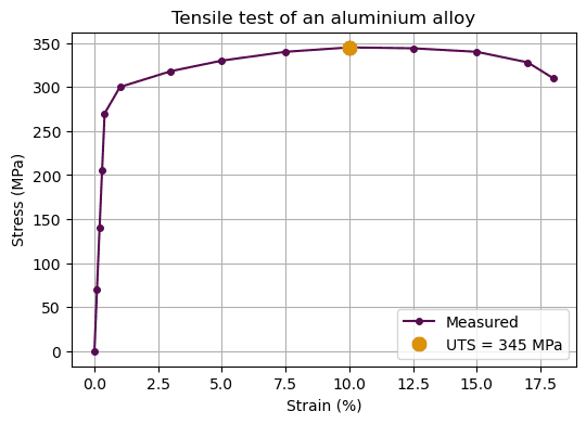
The format string "o" in the second plt.plot() call draws a marker with no line, which is how a single point is highlighted.
Data with a fitted line
When you fit a model, plot the measured points and the fitted line together so the quality of the fit is visible. Calculate the line over a smooth range of x-values with np.linspace() and np.polyval().
import numpy as npimport matplotlib.pyplot as plttemperature = np.array([20, 100, 200, 300, 400, 500]) # °Cstrain = np.array([0.0, 0.00185, 0.00415, 0.00648, 0.00880, 0.01115])coefficients = np.polyfit(temperature, strain, 1)smooth_t = np.linspace(0, 520, 100)plt.figure(figsize=(6, 4))plt.plot(temperature, strain * 100, "o", color="#580A50", label="Measured")plt.plot(smooth_t, np.polyval(coefficients, smooth_t) * 100, "--", color="#DB9000", label=f"Fit: α = {coefficients[0] * 1e6:.1f} × 10⁻⁶ /K")plt.xlabel("Temperature (°C)")plt.ylabel("Thermal strain (%)")plt.title("Thermal expansion")plt.legend()plt.grid(True)plt.show()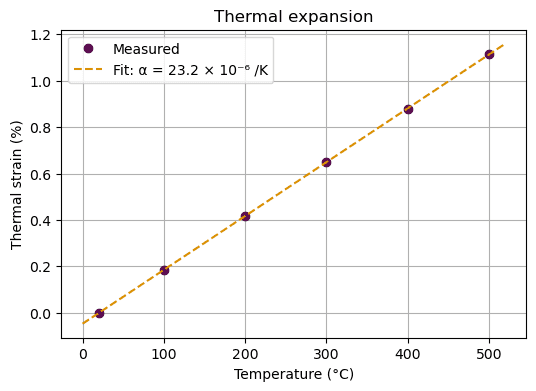
Property charts on logarithmic axes
Material properties span enormous ranges: Young's modulus runs from below 0.01 GPa for foams to over 1000 GPa for diamond. On ordinary axes, most materials would be squashed into one corner. Logarithmic axes, set with plt.xscale("log") and plt.yscale("log"), give equal space to each factor of ten. Charts like this, popularised by Michael Ashby, are a standard tool for choosing materials.
import matplotlib.pyplot as pltfamilies = { "Metals": ([2.7, 4.4, 7.8, 8.9, 19.3], [69, 114, 205, 117, 411]), "Ceramics": ([3.9, 3.2, 2.2, 3.5], [380, 410, 72, 1050]), "Polymers": ([0.95, 1.2, 1.4, 1.05], [1.0, 2.4, 3.0, 3.3]), "Foams": ([0.03, 0.05, 0.1], [0.005, 0.02, 0.08]),} # (density in g/cm³, Young's modulus in GPa)plt.figure(figsize=(6, 4))for family, (density, modulus) in families.items(): plt.scatter(density, modulus, label=family, s=50)plt.xscale("log")plt.yscale("log")plt.xlabel("Density (g/cm³)")plt.ylabel("Young's modulus (GPa)")plt.title("Stiffness versus density")plt.legend()plt.grid(True, which="both", alpha=0.3)plt.show()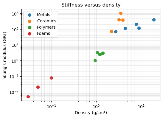
Each material family occupies its own region of the chart, which is exactly what makes these charts useful for selection.
Several plots in one figure
plt.subplots(rows, columns) creates a figure containing a grid of separate plots, called axes. It returns the figure and the axes; you then draw on each axes object directly. Its methods have slightly different names: ax.set_xlabel() instead of plt.xlabel(), and ax.set_title() instead of plt.title().
import numpy as npimport matplotlib.pyplot as plttemperature = np.linspace(300, 1200, 50) # Kdiffusivity = 2.3e-5 * np.exp(-148_000 / (8.314 * temperature))fig, (left, right) = plt.subplots(1, 2, figsize=(9, 3.5))left.plot(temperature, diffusivity, color="#580A50")left.set_xlabel("Temperature (K)")left.set_ylabel("D (m²/s)")left.set_title("Linear scale")right.plot(1000 / temperature, diffusivity, color="#580A50")right.set_yscale("log")right.set_xlabel("1000 / T (1/K)")right.set_title("Arrhenius plot")fig.tight_layout()plt.show()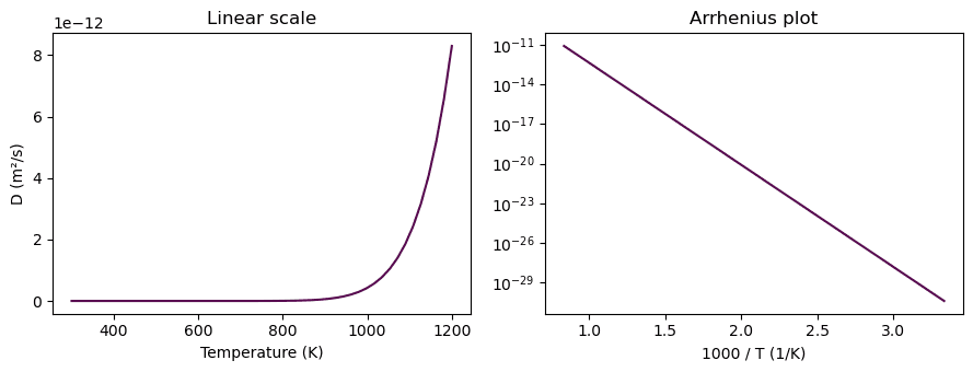
On linear axes the diffusivity looks negligible below about 900 K. The Arrhenius plot (log of D against 1/T) turns the exponential into a straight line whose slope gives the activation energy. Choosing the right axes can reveal the physics.
Knowledge check
Choose an answer and press Check answer. You can retry as often as you like.