Lesson 4 of 4
Introduction to Matplotlib
Draw your first scientific plots with Matplotlib: line plots, scatter plots and bar charts, with labelled axes, titles and legends.
About 30 minutes
In this lesson you will
- Create line and scatter plots with
plt.plot()andplt.scatter() - Label axes, add a title, a legend and a grid
- Plot several data series on one figure
- Choose a suitable plot type for your data
Why plot?
A table of numbers hides trends that a plot reveals at a glance: a linear region, a sudden change, an outlier. Matplotlib is Python's standard plotting library. It can produce anything from a quick check of your data to figures ready for publication. Like NumPy, it has its own SPASCLE course; this lesson covers the essentials.
Most plotting uses the pyplot module, imported as plt by convention. When you run plotting code in SPASCLE's editor, the figure appears in the output panel. The first run takes a little longer while Matplotlib loads.
Your first line plot
plt.plot(x, y) draws a line through the points given by two sequences of the same length: x-coordinates and y-coordinates. Lists and NumPy arrays both work. plt.show() displays the finished figure.
import matplotlib.pyplot as plttemperature = [300, 400, 500, 600, 700, 800] # Kresistivity = [1.72, 2.42, 3.11, 3.81, 4.50, 5.20] # µΩ·cm, copperplt.plot(temperature, resistivity)plt.show()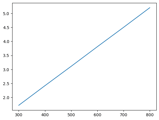
The plot shows the trend, but nobody else could tell what it represents. A scientific plot always needs labelled axes with units.
Labels, titles and grids
| Function | Adds |
|---|---|
plt.xlabel("..."), plt.ylabel("...") | Axis labels |
plt.title("...") | A title above the plot |
plt.grid(True) | Grid lines, which help readers estimate values |
plt.legend() | A key for plots with several series (see below) |
plt.figure(figsize=(w, h)) | A new figure of the given size in inches (call it first) |
plt.plot() also accepts a format for the line and markers. marker="o" adds a circle at each data point, which shows readers where the measurements actually are. linestyle="--" draws a dashed line, and color= sets the colour.
import matplotlib.pyplot as plttemperature = [300, 400, 500, 600, 700, 800]resistivity = [1.72, 2.42, 3.11, 3.81, 4.50, 5.20]plt.figure(figsize=(6, 4))plt.plot(temperature, resistivity, marker="o", color="#580A50")plt.xlabel("Temperature (K)")plt.ylabel("Resistivity (µΩ·cm)")plt.title("Electrical resistivity of copper")plt.grid(True)plt.show()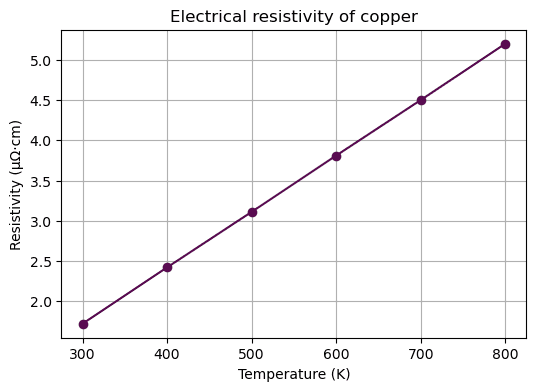
Several series and a legend
Call plt.plot() several times before plt.show() to draw several lines on the same axes. Give each a label=, then call plt.legend() to show which line is which. NumPy is handy here for generating smooth x-values with np.linspace() and calculating y-values from a formula.
import numpy as npimport matplotlib.pyplot as plttemperature = np.linspace(0, 400, 50) # temperature rise, Klength = 1.0 # mfor name, alpha in [("Aluminium", 23.1e-6), ("Copper", 16.5e-6), ("Steel", 12.0e-6)]: expansion_mm = alpha * length * temperature * 1000 plt.plot(temperature, expansion_mm, label=name)plt.xlabel("Temperature rise (K)")plt.ylabel("Expansion of a 1 m bar (mm)")plt.title("Thermal expansion")plt.legend()plt.grid(True)plt.show()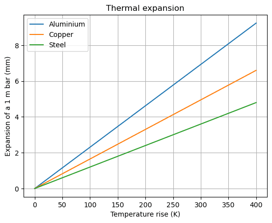
Scatter plots
Use plt.scatter(x, y) when each point is an independent measurement and joining them with a line would suggest a continuity that isn't there, for example when comparing properties of different materials. plt.annotate() adds a text label next to a point.
import matplotlib.pyplot as pltnames = ["Mg", "Al", "Ti", "Fe", "Cu", "W"]density = [1.74, 2.70, 4.51, 7.87, 8.96, 19.25] # g/cm³modulus = [45, 70, 116, 211, 130, 411] # GPaplt.scatter(density, modulus, color="#580A50")for name, x, y in zip(names, density, modulus): plt.annotate(name, (x, y), textcoords="offset points", xytext=(5, 5))plt.xlabel("Density (g/cm³)")plt.ylabel("Young's modulus (GPa)")plt.title("Stiffness versus density of metals")plt.grid(True)plt.show()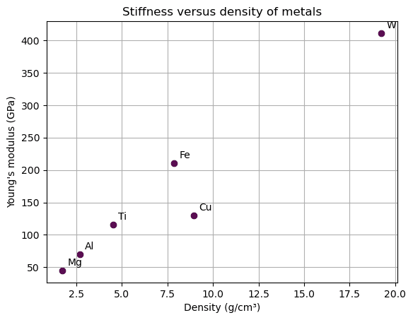
Bar charts
plt.bar(categories, values) compares a quantity across named categories.
import matplotlib.pyplot as pltmetals = ["Al", "Cu", "Fe", "Ti", "W"]melting_point = [660, 1085, 1538, 1668, 3422] # °Cplt.bar(metals, melting_point, color="#580A50")plt.ylabel("Melting point (°C)")plt.title("Melting points of common metals")plt.show()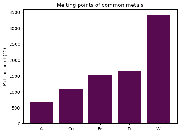
| Plot | Use it for |
|---|---|
Line plt.plot() | A quantity that changes continuously with another: temperature over time, a property against composition, a calculated curve |
Scatter plt.scatter() | Independent measurements, or the relationship between two properties across many samples |
Bar plt.bar() | Comparing one value across separate categories |
Saving figures
On your own computer,
plt.savefig("figure.png", dpi=300) saves the current figure to a file. Call it before plt.show(). Use .pdf or .svg for figures that will be printed or published.Knowledge check
Choose an answer and press Check answer. You can retry as often as you like.